Lab 7: Kalman Filter

In Lab 7, I drove the car at a wall as fast as possible and used the ToF readings to find the steady state speed and implement a Kalman filter in simulation.

Prelab

As part of Lab 5, I had chosen a ToF timing budget of 20 ms, yielding a distance sensing frequency of 50 Hz. Conversely, the position PID controller in that lab was able to run at roughly 280 Hz. To deal with the resulting gaps in distance data, I employed linear extrapolation to predict the intermediate readings in a very simplistic way. In this lab, I turned to the more sophisticated approach of a Kalman filter to implement this same idea of inter-measurement predictions.

Tasks

Task 1: Estimate Drag and Mass

Starting with Newton's second law of motion,

$$F=ma=m\ddot{x},$$

and the linear force on the car in terms of drag $d$ and motor input $u$,

$$F=-d\dot{x}+u,$$

the dynamics of the system can be described by the expression

$$\ddot{x}=-\frac{d}{m}\dot{x}+\frac{u}{m}.$$

Then, representing the state of the system as the vector

$$x=\left[\begin{array}{c}x\\ \dot{x}\end{array}\right],$$

the expression for $\ddot{x}$ can be rewritten in the form $\dot{x}=Ax+Bu$ as

$$\left[\begin{array}{c}\dot{x}\\ \ddot{x}\end{array}\right]=\left[\begin{array}{cc}0& 1\\ 0& -d/m\end{array}\right]\left[\begin{array}{c}x\\ \dot{x}\end{array}\right]+\left[\begin{array}{c}0\\ 1/m\end{array}\right]u.$$

From this system, the drag $d$ and mass $m$ can be estimated for the steady state input $u_{ss}$, the steady state speed ${\dot{x}}_{ss}$, and the 90% rise time $t_{0.9}$ as

$$d=\frac{u_{ss}}{{\dot{x}}_{ss}}m=\frac{-d\cdot t_{0.9}}{\ln (1-d\cdot {\dot{x}}_{ss})}=\frac{-d\cdot t_{0.9}}{\ln (1-0.9)}.$$

To reach steady state and find these quantities for the real car, I used a BLE command to set the motors to 100% input ($u_{ss}=1\text{ N}$) and drive toward a wall as fast as possible while collecting data. To avoid crashing the car, I set all motor pins to HIGH for about a second when the distance to the wall was less than 1 meter, thereby actively braking the car. Because I had taped the wheels for the orientation PID experiments in Lab 6, the car entered a slide when the wheels locked under braking and bumped into the wall anyway, albeit less forcefully than it would have at full motor input.

The data I collected during the wall run is visualized in the plot below.

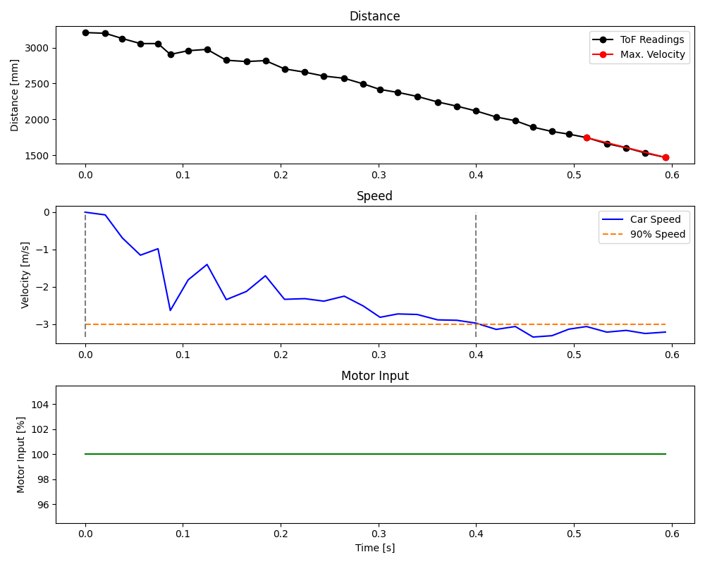
From the distance readings and corresponding timestamps, I found the steady state speed ${\dot{x}}_{ss}$ to be roughly 3.35 m/s, the 90% rise time to be roughly 0.40 s, and the speed at 90% rise time to be 3.01 m/s. Therefore, the drag and mass of the car system are

$$d=\frac{1\text{ N}}{3.35\text{ m/s}}=0.299\text{ kg/s},$$ $$m=\frac{-0.299\text{ kg/s}\cdot 0.40\text{ s}}{\ln (0.1)}=0.0519\text{ kg}.$$

Task 2: Initialize KF

In the state vector form of the system dynamics above, matrices $A$ and $B$ are

$$A=\left[\begin{array}{cc}0& 1\\ 0& -d/m\end{array}\right]=\left[\begin{array}{cc}0& 1\\ 0& -5.76\end{array}\right]B=\left[\begin{array}{c}0\\ 1/m\end{array}\right]=\left[\begin{array}{c}0\\ 19.3\end{array}\right].$$

To implement a Kalman filter for discrete-time distance readings, I discretized these matrices using the following bit of Python.

n = 2 # dimension of the state space
dt = 0.02 # seconds between readings

Ad = np.eye(n) + dt * A
Bd = dt * B

I then defined an observation matrix $C$ such that $y=Cx$, and initialized the state vector $x$ from the first of the ToF distance readings collected earlier.

# Select the relevant part of the data
time = np.array(time[start:end]) - time[start]
tof = tof[start:end]
uss = 1

C = np.array([[-1, 0]])
x = np.array([[-tof[0]], [0]]) # tof from collected data

The last component I needed for the Kalman filter was the process noise and sensor noise covariances. These are defined for the sampling time $dt$ or sensor variance $dx$ by the expressions

$${\sigma }_1={\sigma }_2=\sqrt{\frac{{10}^2}{dt}}{\sigma }_3=\sqrt{\frac{{10}^2}{dx}}.$$

For the process, the sampling time for position and velocity is governed by the ToF sampling period of 20 ms. For the sensor, I assumed uncorrelated noise and estimated that the ToF readings exhibit a variance of roughly 50 mm. From these, I defined the covariances and diagonal covariance matrices ${\mathrm{\Sigma }}_u$ and ${\mathrm{\Sigma }}_z$.

# Process noise
sigma_1 = 70
sigma_2 = 70

# Sensor noise
sigma_3 = 45

Sigma_u = np.array([[sigma_1**2, 0], [0, sigma_2**2]]) # confidence in model
Sigma_z = np.array([[sigma_3**2]]) # confidence in measurements

Task 3: Implement KF in Python

With all definitions and conditions in place, I implemented a kalman() function in Python to perform each step of the filter algorithm.

# Kalman filter step function
def kalman(mu, sigma, u, y, update = True):
    mu_p = Ad.dot(mu) + Bd.dot(u)
    sigma_p = Ad.dot(sigma.dot(Ad.transpose())) + Sigma_u

    if not update:
        return mu_p, sigma_p

    sigma_m = C.dot(sigma_p.dot(C.transpose())) + Sigma_z
    kkf_gain = sigma_p.dot(C.transpose().dot(np.linalg.inv(sigma_m)))

    y_m = y - C.dot(mu_p)
    mu = mu_p + kkf_gain.dot(y_m)
    sigma = (np.eye(2) - kkf_gain.dot(C)).dot(sigma_p)

    return mu, sigma

# Uncertainty for initial state
sigma = np.array([[20**2, 0], [0, 10**2]])

kf = []

i = 0
for t in time:
    # Step through discrete time
    update = time[i+1] <= t
    i += 1 if update else 0

    # Run Kalman filter for each time step
    x, sigma = kalman(x, sigma, uss, tof[i], update)
    kf.append(x[0])

The results of the Kalman filter are shown in the plot below.

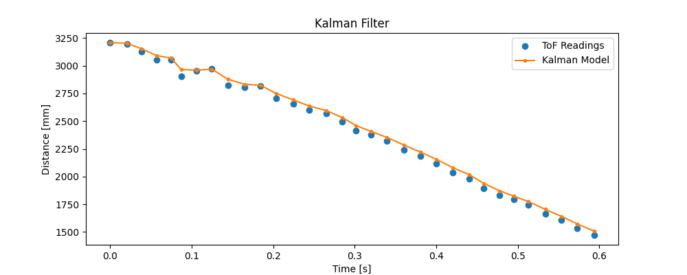
The model above fits the ToF readings fairly well, which suggests that my covariances were decent estimates. If the model had drifted too dramatically from the real measurements, the process covariance would have been too high, as in the following plot.

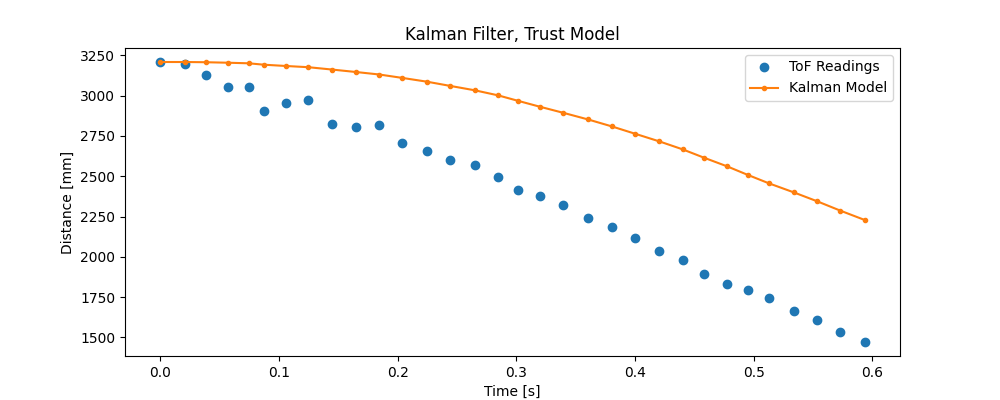
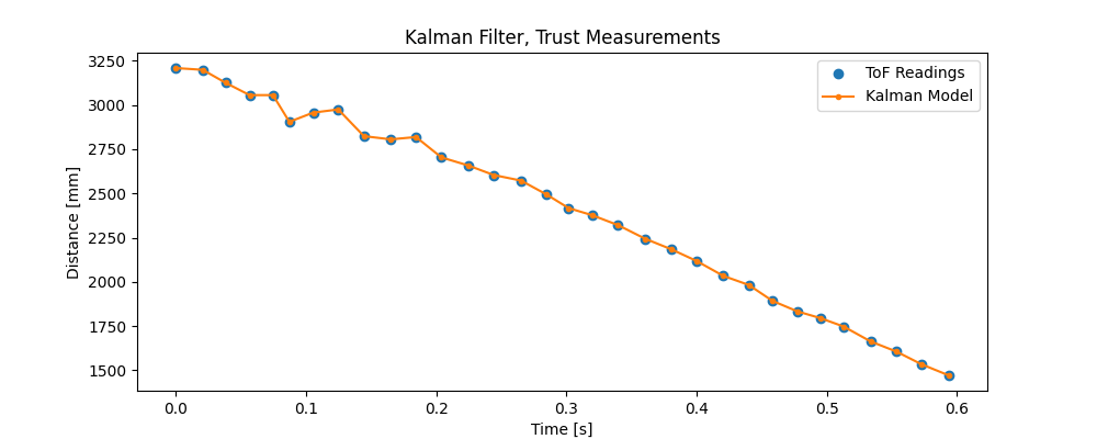
Conversely, if the model had aligned too closely with the somewhat noisy ToF data, the sensor covariance would have been too high, as in the following plot.

Optional 5000-Level: Speeding Up

Running the Kalman filter at the same frequency as the ToF readings works fine, but it would be even more useful to predict ToF behavior between readings, as well. That way, the Kalman filter could replace the linear extrapolation of ToF data from Lab 5. To achieve this, I shortened the sampling time $dt$ and enabled the model's prediction step in the Kalman loop.

 n = 2 # dimension of the state space
!dt = 0.0225 / 4 # seconds between readings
 Ad = np.eye(n) + dt * A
 Bd = dt * B

 ...

 i = 0
!interval = 5 # ms
!steps = np.arange(0, int(time[-1] * 1000), interval) / 1000
!for t in steps:
     # Step through discrete time
     update = time[i+1] <= t
     i += 1 if update else 0

     # Run Kalman filter for each time step
     x, sigma = kalman(x, sigma, uss, tof[i], update)
     kf.append(x[0])

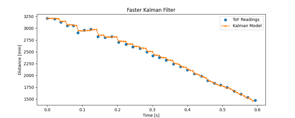
The Kalman output now includes distance values between ToF readings that are fairly representative of the change in physical position of the car as it approached the wall.

Conclusion

This lab has been a great introduction to Kalman filters. I struggled with the concepts at first, but implementing and debugging a practical model for ToF sensor data helped me understand what the filter is actually doing.

Importantly, the Kalman approach is far better than the extrapolation in Lab 5. Below is the relevant plot from that lab for comparison.

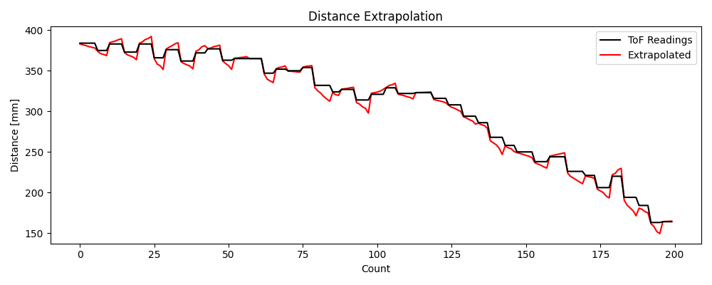
I now plan to implement a Kalman filter on my car for the next lab to replace the spiky interpolation in the position PID controller.