Lab 11: Real Localization – MAE 4190 Fast Robots

In Lab 11, I used the orientation mapping system from Lab 9 and the Bayes filter from Lab 10 to localize the real car in our lab arena.

Simulation

I started the lab by verifying my simulated localization solution from Lab 10 by running lab11_sim.ipynb, one of the provided Lab 11 notebooks. The image below shows the results of the Lab 11 simulation.

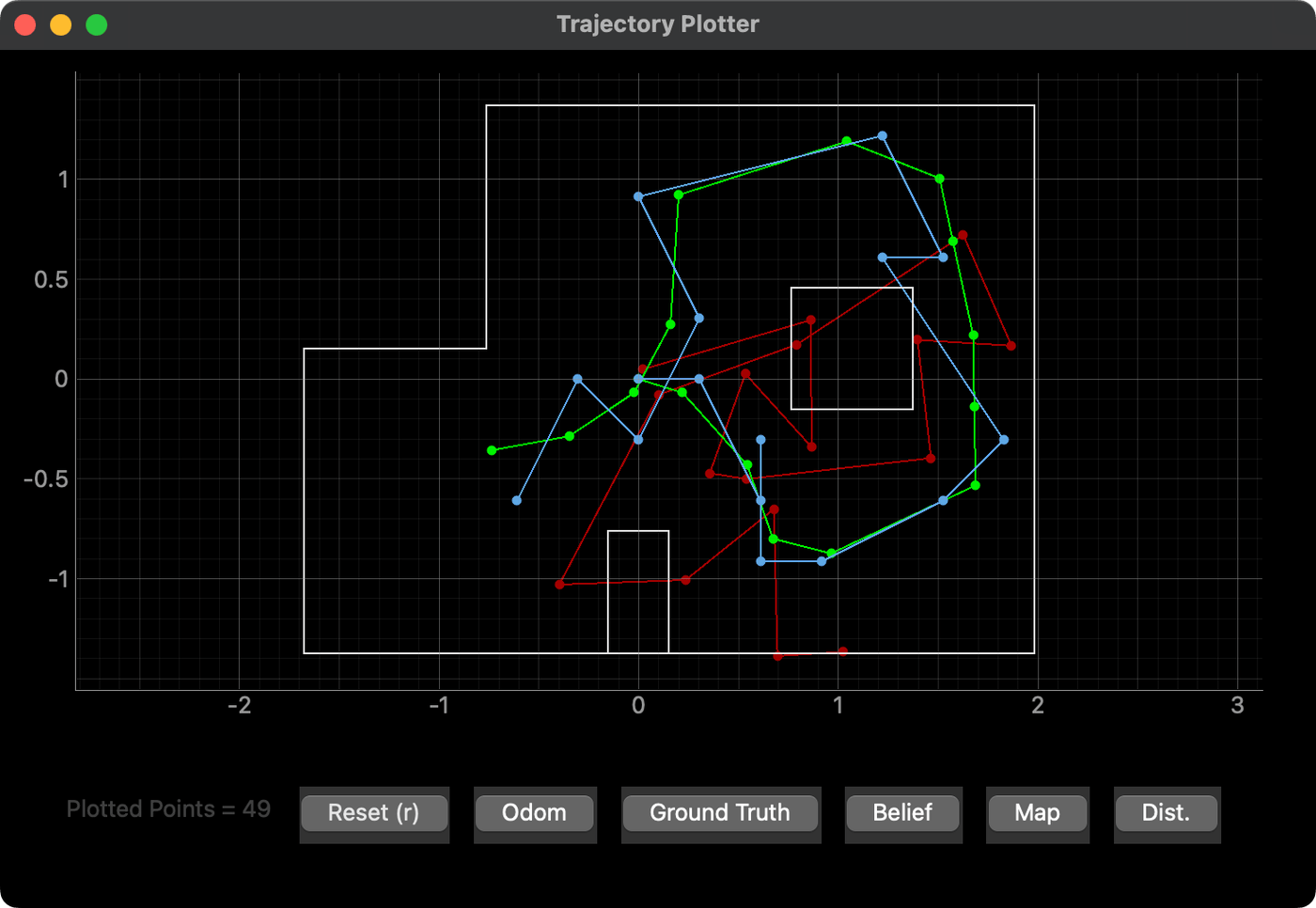
This looks quite similar to what I saw in Lab 10, the video from which is included below for reference. The Lab 11 version took 1:31 to run, while my Lab 10 solution took 1:33. I'd say that's well verified.

Reality

For now, because we don't have a mechanism to determine the ground truth of the car, I implemented only the update step of the Bayes filter with the method perform_observation_loop() in the provided RealRobot class. The method uses BLE to command the car to spin in a circle and scan the map in 20 degree increments, reusing the DO_MAPPING Artemis routine I wrote in Lab 9.

# In RealRobot:
def perform_observation_loop(self, rot_vel=120):
    increment = 360 // self.num_steps
    error = 3
    readings = 5

    self.nano.command(CMD.DO_MAPPING, f'{increment}|{error}|{readings}')

    LOG.info('Observing...')

    # Wait for the command to finish
    duration = self.nano.await_end(0.25, 100)

    LOG.info(f'Finished observing in: {duration}')
    LOG.info('Receiving data...')

    self.nano.command(CMD.SEND_SENSOR_DATA)
    self.nano.collect(0.25, key='Tu')

    LOG.info('Finished receiving data.')

    data = [{k: float(v) for k, v in row.items()} for row in self.nano.data]
    run = {key: np.trim_zeros(np.array([row[key] for row in data])) for key in data[0]}

    imu = run['Yu'] # degrees
    tof = run['D1'] # mm

    trials = len(imu) // self.num_steps

    angle = imu.reshape((self.num_steps, trials)).mean(axis=1)[np.newaxis].T
    distance = tof.reshape((self.num_steps, trials)).mean(axis=1)[np.newaxis].T / 1000 # mm -> m

    # Pass all but the last item in each column vector
    return distance, angle

Note my use of a helper function, await_end() which uses asyncio.sleep() to wait for a BLE signal indicating the completion of the mapping command.

Then, in the absence of an automated ground truth, I used the following four marked arena locations from Lab 9 as known poses and ran the update step at each of them:

(-3, -2) ft
(0, 3) ft
(5, -3) ft
(5, 3) ft

Results

Below are the results for each marked location. The green dot in each plot is the ground truth, added manually in Python for each placement of the car. The blue dot is the belief after the Bayes update step.

Marked Pose (-3, -2)

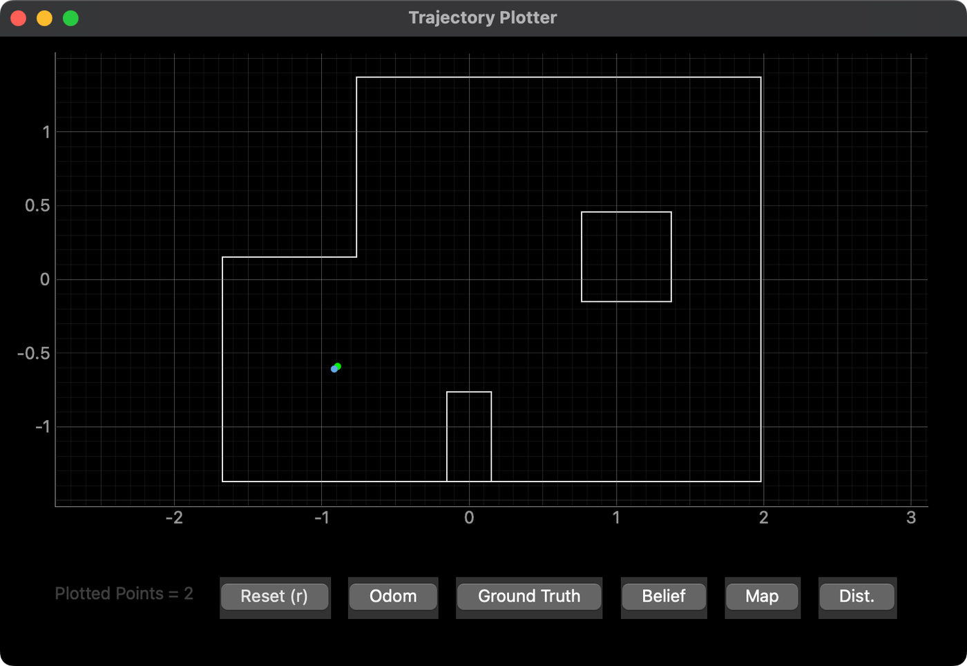
The geometry of this part of the map seemed to yield really good results. I tried this location more than once and the belief was accurate each time. The arena is discretized, so the belief is rounded to some extent, but the result is nevertheless dead on.

Marked Pose (0, 3)

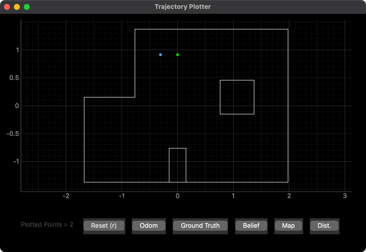
This pose was slightly less accurate. The Bayes filter seemed to weigh the closer readings of the nearest walls more favorably, perhaps because the farther readings were more noisy.

Marked Pose (5, -3)

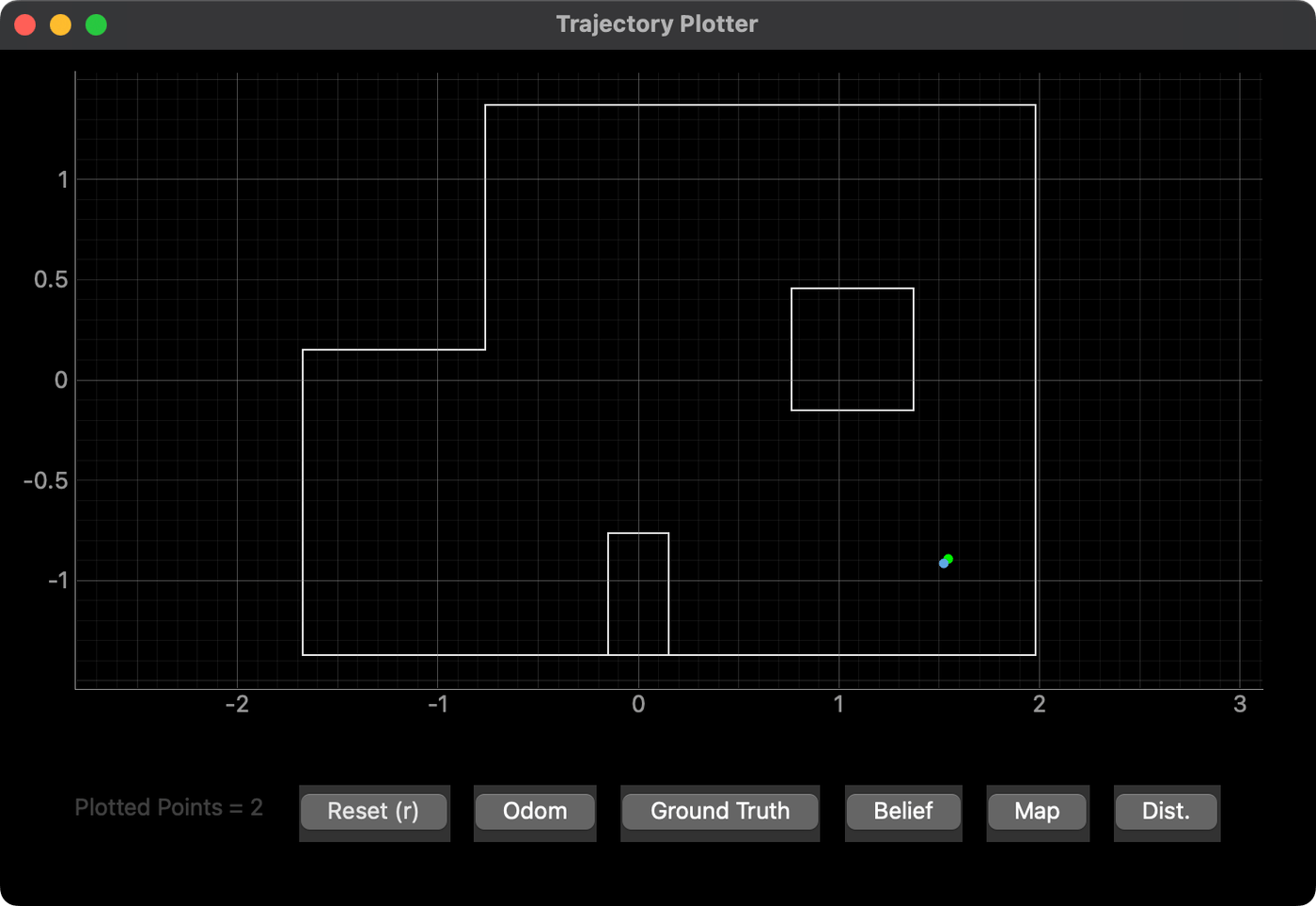
This position was inconsistent. Shown here is a very good result, but I had two others that were slightly off. I think the inconsistency comes from the much more open nature of this part of the arena.

Marked Pose (5, 3)

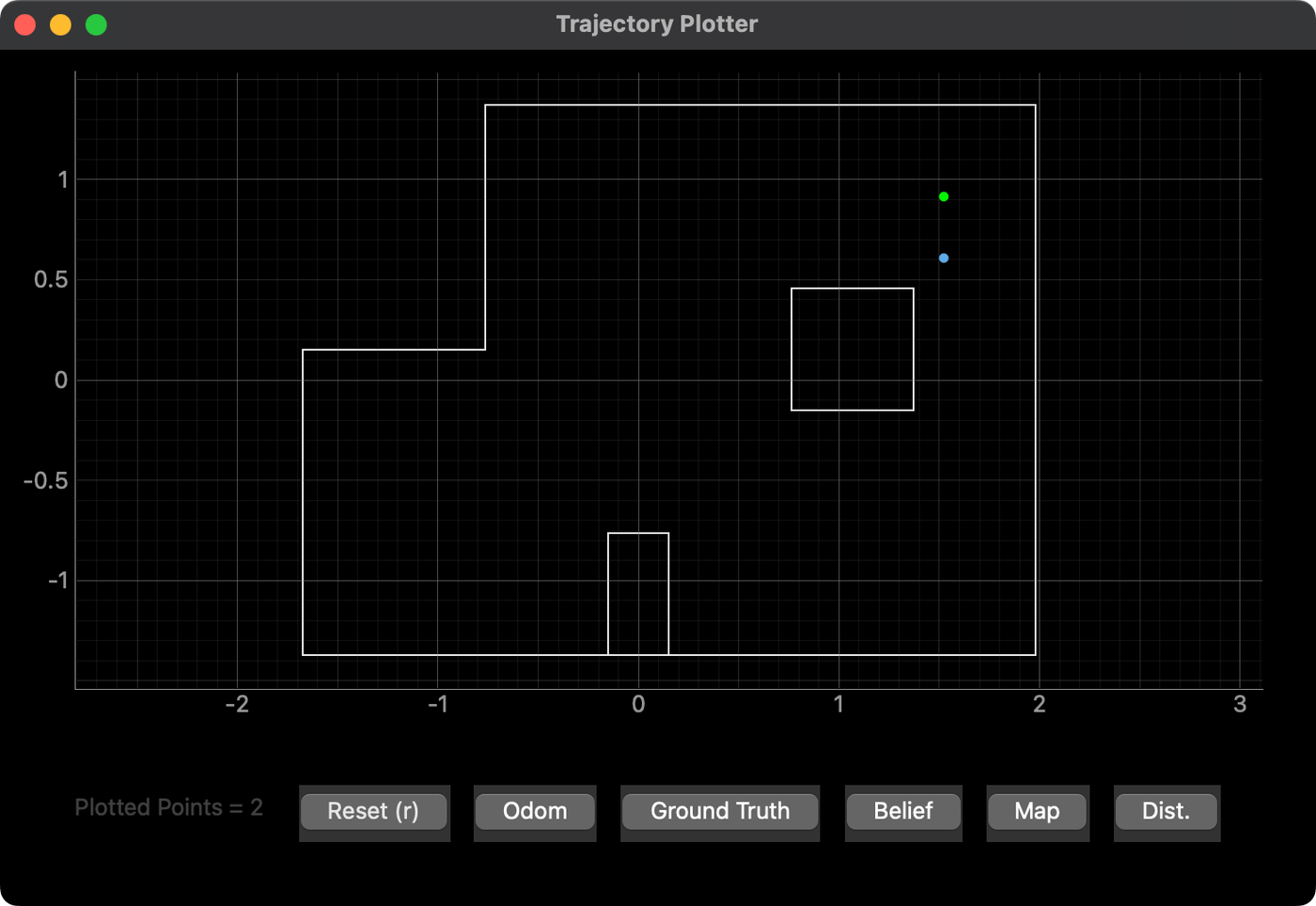
Lastly, this pose, similar to (0, 3), was a bit off the ground truth. Again, I think the dramatic difference between closer and farther walls might be the cause. There may also be a contribution from a discrepancy in the exact positions of the walls of the inner island feature, which, in the physical lab space, is actually a large cardboard box that's slightly undersized and doesn't quite match the grid.

Additional Tests

As extra examples, I tried placing the car at the origin of the map and at (-1.5, -3.5). The results are shown below. The belief still matches the ground truth fairly well in these locations, which supports the robustness of the Bayes filter.

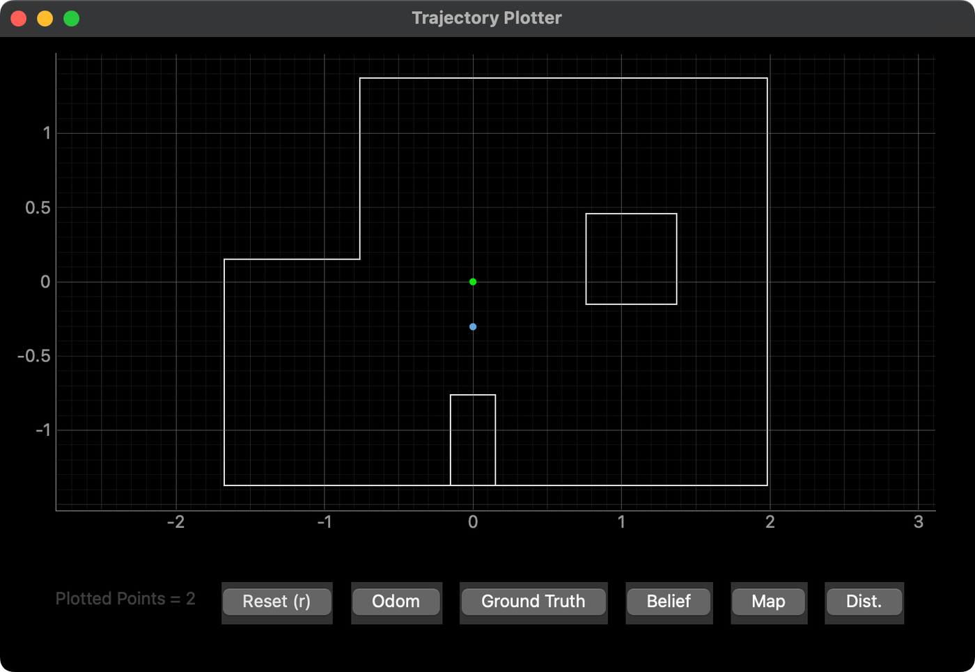
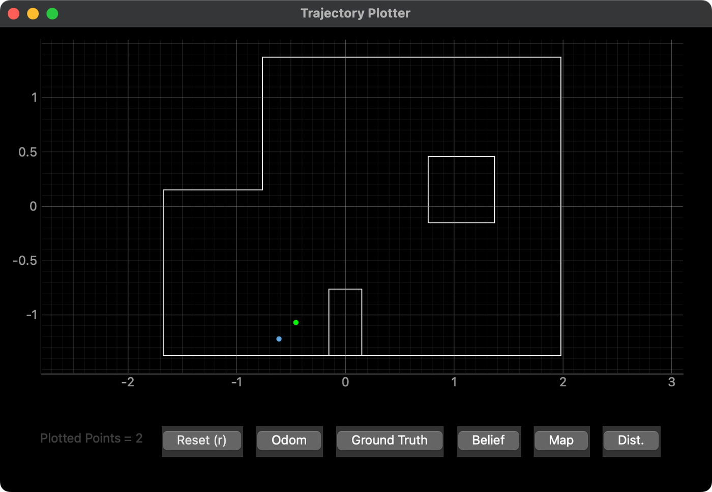
Overall, the Bayes filter seemed to fair much better in geometrically distinct locations. Some of the locations may look similar from the car's perspective due to the subtle symmetry built into the arena. The filter also seemed to prefer regions that are more closed off. Anytime that a significant portion of the measurements approached the limits of the ToF sensors' range—even in long-distance mode—the resulting noise caused minor inconsistencies or inaccuracies in the calculated beliefs.

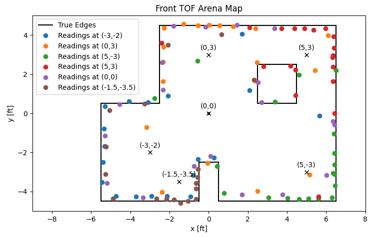
As a last check, I also repeated the mapping process from Lab 9 using the data I collected during localization. The resulting map is shown below.

Demonstration

The following video shows one of the update steps in action at (-3, -2).

Conclusion

This lab was an important step in bringing together many of the systems and principles we've been working toward all semester. In our last lab, we will use the localization process to plan and execute a path through the arena, so it's very encouraging to see such good results from the tests above.