Lab 9: Mapping – MAE 4190 Fast Robots

In Lab 9, I used orientation control to map the edges of a physical space by incrementally taking TOF distance readings from several positions.

Orientation Control

For the mapping routine, I chose orientation control because my PID controller, powered by the IMU's DMP chip, has proven powerful and reliable by now. I would much sooner trust the angles the DMP reports than the TOF sensor readings I would get if I spun the robot continuously. I also decided on angular increments of 15 degrees, giving me 24 distinct orientations per scanning location in the arena.

To implement orientation-based scans of the arena, I added a DO_MAPPING BLE command to the Artemis.

// In handle_command():
case DO_MAPPING: {
    int increment;
    success = robot_cmd.getNextValue(increment);
    if (!success) return;

    int error;
    success = robot_cmd.getNextValue(error);
    if (!success) return;

    int readings;
    success = robot_cmd.getNextValue(readings);
    if (!success) return;

    clearImuData();
    flag_record_imu = false;

    clearTofData();
    flag_record_tof = false;

    // Step through 360 degrees by the given increments
    for (int angle = 0; angle < 360; angle += increment) {
        setOriTarget(angle);

        do {
            // Read yaw from the IMU and run PID control until
            // the angular error is below the given threshold
            readDmpData();
            pidOriControl();
        } while (abs(current_error) >= error);

        idleMotors();

        // Take the given number of yaw and distance readings
        for (int i = 0; i < readings; i = i) {
            if (!TOF1.checkForDataReady() || !TOF2.checkForDataReady()) continue;

            // Enable yaw recording and take a reading,
            // btu bail out if the DMP is not ready yet
            flag_record_imu = true;
            if (!readDmpData()) continue;
            flag_record_imu = false;

            // Enable distance recording and take readings
            flag_record_tof = true;
            readTof1Data();
            readTof2Data();
            flag_record_tof = false;

            i++;
        }
    }

    // End the routine
    idleMotors();
    flag_pid_ori = false;

    break;
}

This command sequentially points the car in each of the desired orientations by calling the PID controller repeatedly until an upper bound on the angular error is achieved, and then takes a desired number of TOF distance readings while the car is stationary. When calling the command in Python, I specified a step size of 15 degrees, an error bound of 4 degrees, and 5 readings at each orientation. This yielded 120 data points per scanning location in the arena.

While testing the command, I tuned the orientation PID gains to achieve fairly decent on-axis turns throughout the entire 360 sweep ( $K_{p}$ of 2.5, $K_{i}$ of 0.25, and $K_{d}$ of 2.5). A demonstration of this is shown in the video below.

Despite my efforts, the turns were not flawless; there was about 2 inches of drift from start to end of the mapping routine. Therefore, I would expect the same 2 inches of maximum error in the map. On average, this would then be roughly 1 inches of error around the perimeter of an empty 4x4-meter room.

Readings

With the mapping command ready, I placed my car in each of four designated locations in the arena, being careful to use the same absolute initial orientation every time. The four locations are given as coordinates relative to the origin in the middle of the arena and based on the 1x1-foot tile grid in the floor.

(-3, -2) ft
(5, 3) ft
(0, 3) ft
(5, -3) ft

The video below shows the mapping routine in action at (-3, 2).

After taking distance measurements from each location, I sent the collected data over BLE to use for plotting later.

The car's overall behavior during the scans gave me confidence that the map data would be of fairly high quality. The incremental turns were consistent and snappy, and the repeated readings for each orientation were relatively close.

To check the raw results of the mapping routines, I plotted the averages of the data for each arena location on polar axes. From the visualizations, the readings generally match with what I would expect: a clear pattern along the closest boundaries, with a less certain trend in more empty space.

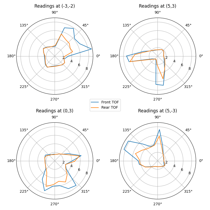
Because the two TOF sensors are mounted opposite each other at the front and rear of my car, performing a 360 sweep completes two scans that are out of phase by 180 degrees. When aligned, these seem to match up quite well, although the rear TOF appears more limited in range. This may be due to a slight downward angle of the rear sensor, causing it to pick up the floor at sufficient distance from the car.

Transformations

Next, I converted the distance measurements taken relative to the car at each scan location into the arena's global reference coordinates ( $x$ and $y$ ). I did this by defining a three-dimensional transformation matrix $T$ , such that

$T = [\begin{matrix} R & d \\ 0 & 1 \end{matrix}] = [\begin{matrix} \cos (θ) & - \sin (θ) & x \\ \sin (θ) & \cos (θ) & y \\ 0 & 0 & 1 \end{matrix}],$

and two position vectors $P_{1}$ and $P_{2}$ for the TOF sensors relative to the center of the car, such that

$P_{1} = [\begin{matrix} {TOF}_{1} \\ 0 \\ 1 \end{matrix}] P_{2} = [\begin{matrix} - {TOF}_{2} \\ 0 \\ 1 \end{matrix}] .$

In my case, the front sensor ${TOF}_{1}$ is located about 2.5 inches front of center, while the rear sensor ${TOF}_{2}$ is located about 3 inches rear of center. I applied these offsets to the distances measured by each sensor during mapping, and transformed the final distances into the global arena coordinates.

When all the data is plotted together, the result of this process is a map of the arena as seen by two TOF sensors at four different scanning locations, each with their own quirks.

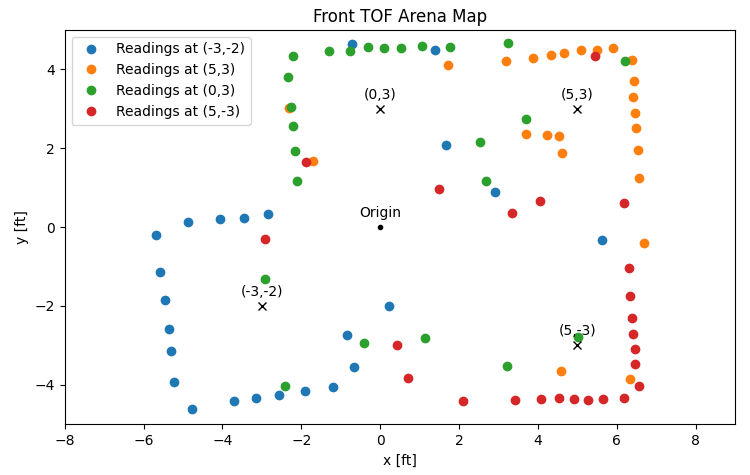
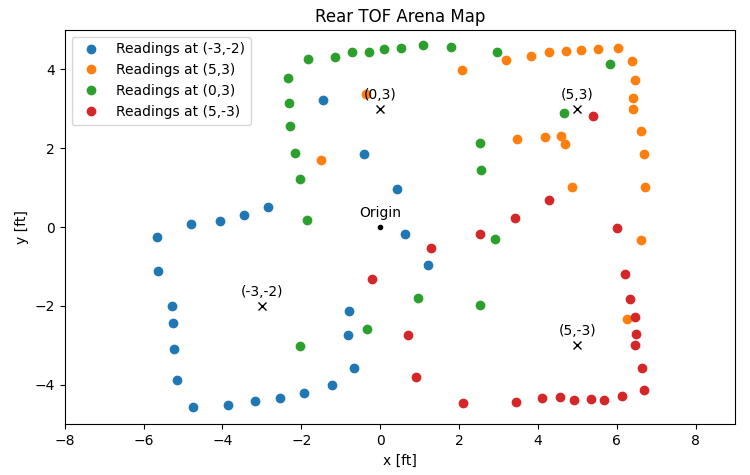
From these plots, I can tell, as before, that the two TOF sensors are quite similar, but that the rear sensor is a bit more limited in range or perhaps simply a bit more noisy than the front sensor. The resulting map is cleaner when considering only the front TOF sensor's measurements.

Edges

To illustrate the accuracy of the maps, I drew lines to estimate the edges detected by the TOF sensors as well as the true edges of the arena. The estimated and true cases line up nicely because I corrected for small angular offsets between the four sets of measurements. The need for these offsets comes from slight differences in how I placed the car down, how the DMP self-calibrated its zero-point during startup, and how patient I was in letting my PID controller settle into its initial orientation before starting the incremental turns.

The angular corrections for each set of measurements were 8, 5, 4, and 2 degrees, respective to the order of locations listed earlier. These were added to each location's angular readings to align them to the $x$ - $y$ coordinate system.

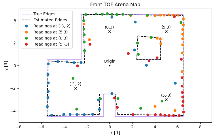
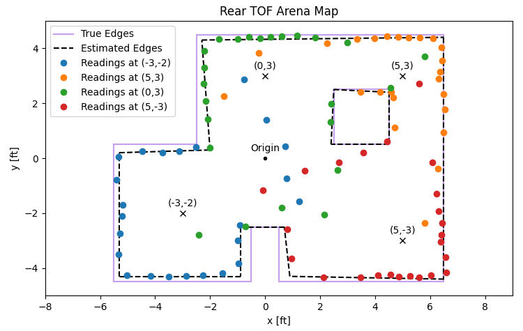
The end points of the estimated edges, as $(x, y)$ pairs, form a line-based map that can be used in future simulations.

# (x_start, y_start) pairs
starts = [(-0.9, -4.3), (-5.5, -4.4), (-5.4, 0.4), (-2.2, 0.2), (-2.3, 4.5), (6.5, 4.4), (6.5, -4.4), (0.7, -4.3), (0.5, -2.5), (-0.9, -2.5), (4.5, 0.5), (2.4, 0.5), (2.5, 2.6), (4.5, 2.4)]

# (x_end, y_end) pairs
ends = [(-5.5, -4.4), (-5.4, 0.4), (-2.2, 0.2), (-2.3, 4.5), (6.5, 4.4), (6.5, -4.4), (0.7, -4.3), (0.5, -2.5), (-0.9, -2.5), (-0.9, -4.3), (2.4, 0.5), (2.5, 2.6), (4.5, 2.4), (4.5, 0.5)]

Conclusion

This lab was quite satisfying. After all the work that I've put into my car, it was nice to see it be able to perform a task like mapping a physical space and finding the edges and obstacles. From here, I imagine we'll be tasked with localizing and navigating within a map, which will bring the car that much closer to proper autonomous control and decision-making.