Lab 10: Simulated Localization – MAE 4190 Fast Robots

In Lab 10, I used a Python simulation to localize a virtual robot in a 2D environment similar to the arena set up in our lab space.

Localization and Bayes Filtering

Robots like our cars have no absolute or "true" knowledge of their position, so we must use information about the robot's environment to infer a position. This process is known as localization, and works best when built on probability.

To achieve probabilistic localization, we use a Bayes filter, which operates on a "belief". From its sensors and control inputs, and based on an initial state, a robot will have some idea of where it is; this is the belief. As the robot gets new sensor readings and control inputs, it can update that belief according to Bayesian inference.

Our robot's state represents its position on the ground plane in $x$ and $y$ coordinates, and its orientation $θ$ in that plane. The robot's orientation is given in angles between -180 and 180 degrees. The bounds of the ground plane are the same as the arena we used in Lab 9, without outer limits:

–5.5 ft $\leq x <$ 6.5 ft
–4.5 ft $\leq y <$ 4.5 ft

The continuous 3D space the robot can occupy is discretized into a grid such that each cell represents 1x1 ft of planar space and 20 degrees of orientation. The grid is thus a 12x9x18 volume of cells.

Algorithm

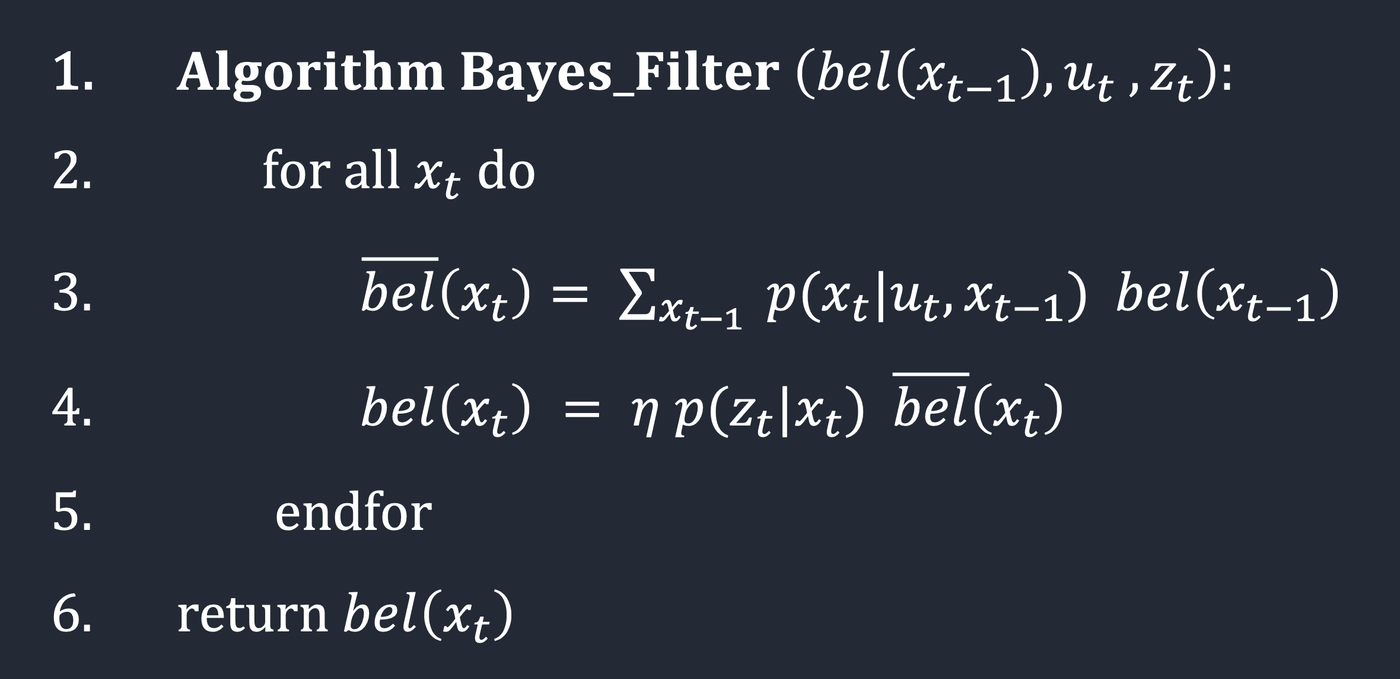
The Bayes filter is an iterative process that first predicts the robot's next position based on control inputs, then updates that position using sensor observations. The prediction step increases uncertainty in the belief, while the update step decreases uncertainty. This algorithm is outlined in the following screenshot from Lecture 17.

Here, $bel (x_{t - 1})$ is the previous belief represented as a 3D matrix where each element is the probability that the robot is located in the corresponding grid cell, $u_{t}$ is the current control input that caused the change in pose $x_{t - 1}$ to $x_{t}$ , and $z_{t}$ is the current sensor state of 18 readings in 20 degree increments.

The algorithm loops over all possible poses $x_{t}$ in the form ( $x$ , $y$ , $θ$ ) at the current point in time. With each iteration, we first estimate a new belief by multiplying the probability of the previous state by the probability of the new state. The sum of all state multiplications forms the predicted belief $\overset{―}{bel} (x_{t})$ . We then update the belief by multiplying it by the probability of obtaining the sensor readings in the current pose and normalizing via the factor $η$ to get $bel (x_{t})$ .

Sensor and Motion Models

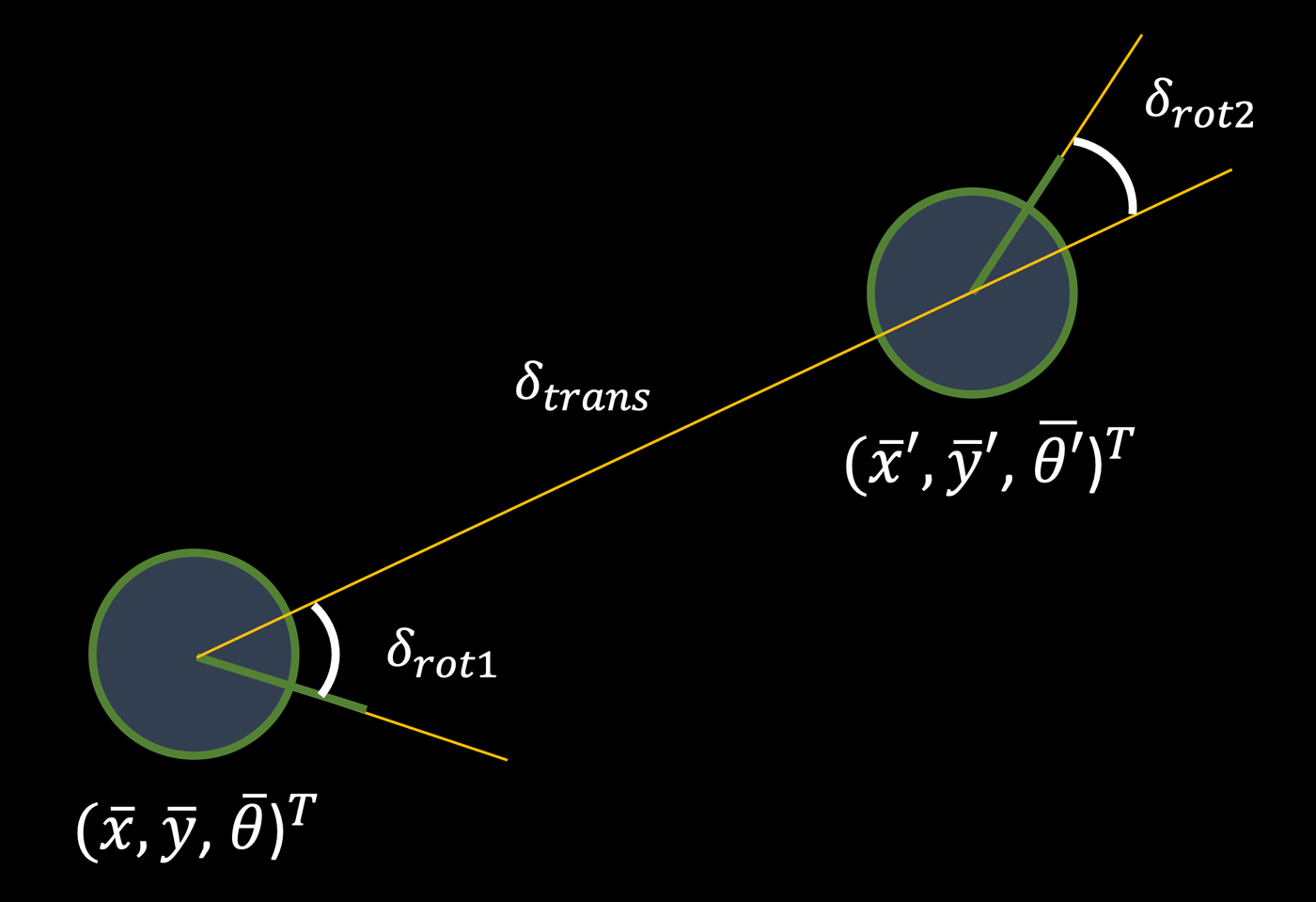
The robot's sensors are modeled to have a Gaussian distribution of noise. The control inputs follow an odometry motion model. The odometry model describes the difference between two positions or "poses" as an initial rotation, a translation, and a final rotation. This model is visualized in the diagram below.

Tasks

Using the provided Python simulation and Lab 10 notebook, I wrote the following functions to implement the Bayes filter.

Compute Control

The compute_control() function takes in a current pose and a previous pose and, using their difference, determines the initial rotation, translation, and final rotation that make up the steps of the odometry model, such that

$δ_{rot1} = \arctan ({\bar{y}}^{'} - \bar{y}, {\bar{x}}^{'} - \bar{x}) - \bar{θ}$ $δ_{trans} = \sqrt{({\bar{y}}^{'} - \bar{y})^{2} + ({\bar{x}}^{'} - \bar{x})^{2}}$ $δ_{rot2} = {\bar{θ}}^{'} - \bar{θ} - δ_{rot1} .$

In Python, $\arctan ()$ is achieved using NumPy's arctan2, whose output is converted from radians to degrees using degrees(), and $δ_{trans}$ is calculated using NumPy's hypot(), which requires less syntax than a manual square root expression. Both angles are additionally normalized to [–180, 180].

def compute_control(cur_pose, prev_pose):
    """ Given the current and previous odometry poses, this function extracts
    the control information based on the odometry motion model.

    Args:
        cur_pose  ([Pose]): Current Pose
        prev_pose ([Pose]): Previous Pose

    Returns:
        [delta_rot_1]: Rotation 1  (degrees)
        [delta_trans]: Translation (meters)
        [delta_rot_2]: Rotation 2  (degrees)
    """
    # Get position and rotation components from current and previous poses
    cur_x, cur_y, cur_theta = cur_pose
    prev_x, prev_y, prev_theta = prev_pose

    # Calculate the first rotation, then normalize to (-180, 180)
    delta_rot_1 = mapper.normalize_angle(
        np.degrees(np.arctan2(cur_y - prev_y, cur_x - prev_x)) - prev_theta,
    )

    # Calculate the translation as a hypotenuse
    delta_trans = np.hypot(cur_y - prev_y, cur_x - prev_x)

    # Calculate the second rotation, then normalize to (-180, 180)
    delta_rot_2 = mapper.normalize_angle(cur_theta - prev_theta - delta_rot_1)

    return delta_rot_1, delta_trans, delta_rot_2

Odometry Motion Model

The odom_motion_model() function takes in a current pose and a previous pose, extracts the odometry model parameters from them using compute_control(), and then calculates the probabilities of those parameters as Gaussian distributions with relevant provided standard deviation $σ$ and centered on the control input u.

def odom_motion_model(cur_pose, prev_pose, u):
    """ Odometry Motion Model

    Args:
        cur_pose  ([Pose]): Current Pose
        prev_pose ([Pose]): Previous Pose
        (rot1, trans, rot2) (float, float, float):
            A tuple with control data in the format (rot1, trans, rot2)
            with units (degrees, meters, degrees)

    Returns:
        prob [float]: Probability p(x'|x, u)
    """
    # Get control parameters from the current and previous poses
    delta_rot_1, delta_trans, delta_rot_2 = compute_control(cur_pose, prev_pose)

    # Determine the probabilities of the control parameters
    prob_rot_1 = loc.gaussian(delta_rot_1, u[0], loc.odom_rot_sigma)
    prob_trans = loc.gaussian(delta_trans, u[1], loc.odom_trans_sigma)
    prob_rot_2 = loc.gaussian(delta_rot_2, u[2], loc.odom_rot_sigma)

    return prob_rot_1 * prob_trans * prob_rot_2

Prediction Step

The prediction_step() function takes in a current and previous odometry state, extracts the odometry model parameters, and then iterates over the entire grid of discretized cells for both the previous and current pose to construct a predicted belief $\overset{―}{bel}$ from odom_motion_model(). The probabilities are multiplied together for each cell, tallied for the entire grid, and finally normalized as a distribution to sum to 1.

Because of the large number of iterations required to cover the 3D simulation volume, we can speed up the process a bit by ignoring very small probabilities less than 0.0001, which don't contribute significantly to the belief. This lowers the accuracy of the filter but decreases computational cost.

def prediction_step(cur_odom, prev_odom):
    """ Prediction step of the Bayes Filter.
    Update the probabilities in loc.bel_bar based on loc.bel from the previous time step and the odometry motion model.

    Args:
        cur_odom  ([Pose]): Current Pose
        prev_odom ([Pose]): Previous Pose
    """
    # Get control parameters from odometry
    u = compute_control(cur_odom, prev_odom)

    # Initialize bel bar
    loc.bel_bar = np.zeros((mapper.MAX_CELLS_X, mapper.MAX_CELLS_Y, mapper.MAX_CELLS_A))

    # Loop over the entire grid
    for prev_x in range(mapper.MAX_CELLS_X):
        for prev_y in range(mapper.MAX_CELLS_Y):
            for prev_theta in range(mapper.MAX_CELLS_A):
                # Skip states with very low probabilities to speed up the prediction
                if (loc.bel[prev_x, prev_y, prev_theta] < 0.0001): continue

                for cur_x in range(mapper.MAX_CELLS_X):
                    for cur_y in range(mapper.MAX_CELLS_Y):
                        for cur_theta in range(mapper.MAX_CELLS_A):
                            # Calculate the transition probability
                            p = odom_motion_model(
                                mapper.from_map(cur_x, cur_y, cur_theta),
                                mapper.from_map(prev_x, prev_y, prev_theta),
                                u
                            )

                            # Keep running sum of bel_bar
                            loc.bel_bar[cur_x, cur_y, cur_theta] += p * loc.bel[prev_x, prev_y, prev_theta]

    # Normalize bel bar
    loc.bel_bar /= np.sum(loc.bel_bar)

Sensor Model

The sensor_model() function takes in an array of observations and calculates the probabilities of each of these occurring for the current state as a Gaussian distribution and a provided standard deviation $σ$ .

def sensor_model(obs):
    """ This is the equivalent of p(z|x).

    Args:
        obs ([ndarray]): A 1D array consisting of the true observations for a specific robot pose in the map

    Returns:
        [ndarray]: Returns a 1D array of size 18 (=loc.OBS_PER_CELL) with the likelihoods of each individual sensor measurement
    """
    # Calculate the probabilities of the given observations
    return [loc.gaussian(obs[i], loc.obs_range_data[i], loc.sensor_sigma)
        for i in range(mapper.OBS_PER_CELL)]

Update Step

Lastly, the update_step() function iterates over the grid for the current state, retrieves the sensor model data using sensor_model(), and then updates the belief $bel$ . This updated belief is then normalized to sum to 1 and represents the robot's estimation of its position in the discretized environment.

def update_step():
    """ Update step of the Bayes Filter.
    Update the probabilities in loc.bel based on loc.bel_bar and the sensor model.
    """
    # Loop over the grid
    for cur_x in range(mapper.MAX_CELLS_X):
        for cur_y in range(mapper.MAX_CELLS_Y):
            for cur_theta in range(mapper.MAX_CELLS_A):
                # Get the sensor model and update the belief
                p = sensor_model(mapper.get_views(cur_x, cur_y, cur_theta))
                loc.bel[cur_x, cur_y, cur_theta] = np.prod(p) * loc.bel_bar[cur_x, cur_y, cur_theta]

    # Normalize bel
    loc.bel /= np.sum(loc.bel)

Simulation

The first video below shows a trajectory and localization simulation without a Bayes filter. Here, the deterministic odometry model is plotted in red while the ground truth tracked by the simulator is plotted in green. As the simulation runs, it quickly becomes clear that the odometry model on its own is, quite simply, terrible, happily wandering outside of the bounds of the map and making just about no sense at all.

The next video shows the result of adding a Bayes filter to the localization simulation. While the direct odometry model is still less than useless, the probabilistic belief, plotted in blue, gives a very close—and importantly, very applicable—approximation for the robot's true position. The probabilistic approach is especially strong near walls, where the sensor data is more consistent and therefore more trustworthy, and less strong in more open spaces, such as the center of the map.

Conclusion

This lab has demonstrated the importance of using probabilistic models in controls and estimation. When considering how our ToF distance sensors alone can yield quite a range of values as influenced by noise, ambient lighting, surface properties, and so on, it certainly doesn't seem like a good idea to trust these readings directly all of the time. It does indeed make far more sense to assign a probability to everything and use those "weights" to make more reasonable—or perhaps, skeptical—inferences and decisions about an environment filled with uncertainty for a robot with only a couple of low-resolution sensors.