Lab 2: Inertial Measurement Unit

In Lab 2, I configured an inertial measurement unit (IMU) and used its accelerometer and gyroscope to compute pitch, roll, and yaw.

Tasks

Task 1: Set Up the IMU

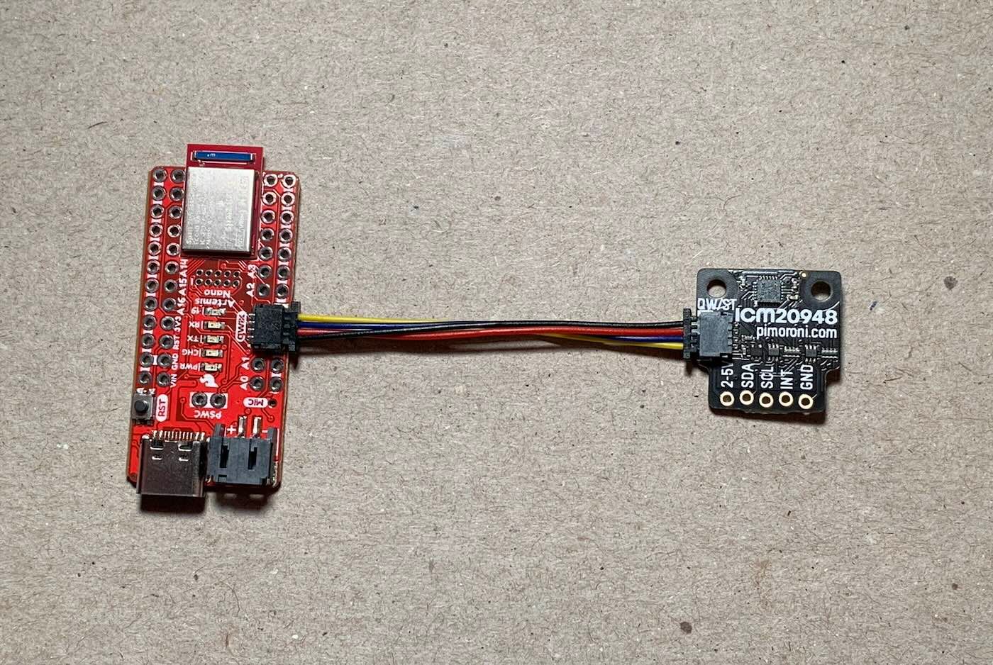
I started the lab by connecting the Pimoroni IMU breakout board to my Artemis using the Qwiic connection and installing SparkFun's ICM 20948 Arduino library.

A diagram on the back of the breakout board shows the IMU coordinate system.

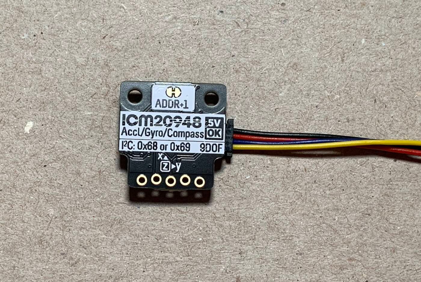
To test the IMU, I ran SparkFun's example sketch, Examples > ICM 20948 > Arduino > Example1_Basics, which outputs data from the accelerometer, gyroscope, and magnetometer to the serial monitor. The macro AD0_VAL, defined near the top of the IMU example sketch, represents the last bit of the IMU's I²C address. I set this to 0 because the ADDR jumper on the Pimoroni board is closed.

The accelerometer measures accelerations relative to the direction of gravitational acceleration $g$, while the gyroscope measures change in angle per unit time in relation to the "zero" state at IMU startup. To read gyroscope data in degrees, the angular rate needs to be integrated over time.

Task 2: Accelerometer

The accelerometer yields readings in the $x$, $y$, and $z$ axes of the coordinate system indicated on the IMU. To calculate pitch $\theta$ and roll $\varphi$ from these values, I implemented the following equations on the Artemis.

$${\theta }_a=atan2(a_x,a_z)$$ $${\varphi }_a=atan2(a_y,a_z)$$

ac_pitch = atan2(IMU.accX(), IMU.accZ()) * 180 / M_PI;
ac_roll = atan2(IMU.accY(), IMU.accZ()) * 180 / M_PI;

I tested the calculations by first holding the IMU level (normal to $g$), then orienting it to induce pitches and rolls of -90 and 90 degrees. Plotting the data, it appears that the IMU is correctly able to identify these orientations.

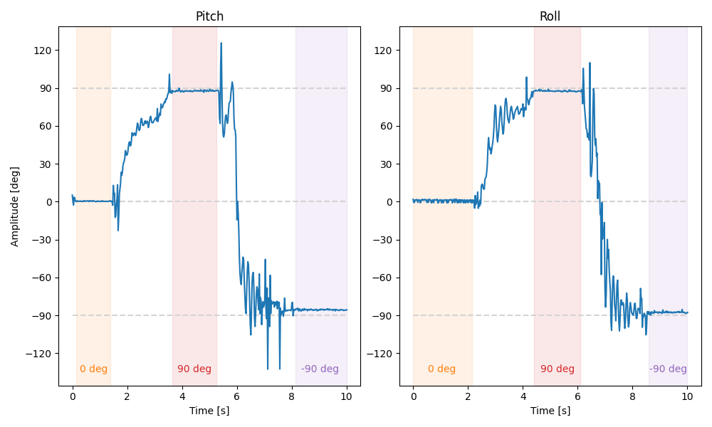
In the plot above, the highlighted regions indicate times when the IMU was pressed flush against the top (0 degrees) or sides (–90/90 degrees) of my desk. The results suggest that the accelerometer is already quite accurate and that two-point calibration is unnecessary.

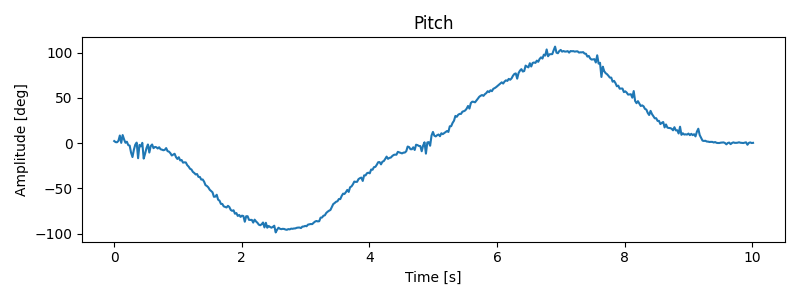
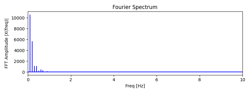
To account for noise in the accelerometer data, I recorded periodic tilting of the IMU, transferred the data over Bluetooth, and performed a Fourier spectrum analysis using SciPy's fft() to identify the periodicity in the signal. From the frequency spectrum, and while considering my sampling frequency of roughly 50 Hz, I chose a safe low-pass filter cutoff frequency $f_c$ of 5 Hz.

A low-pass complimentary filter is defined by the equations:

$${\theta }_{\text{LPF}}[n]=\alpha {\theta }_{\text{raw}}+(1-\alpha ){\theta }_{\text{LPF}}[n-1]$$ $${\theta }_{\text{LPF}}[n-1]={\theta }_{\text{LPF}}[n]$$

Here, $\alpha$ is a weighting coefficient that relates to the sampling period $T$:

$$\alpha =\frac{T}{T+RC}$$ $$f_c=\frac{1}{2\pi RC}$$

Given my sample period of 20 ms and my choice of 5 Hz for $f_c$, I calculated $\alpha$ to be roughly 0.38.

I then implemented the low-pass filter on the Artemis.

#define ALPHA 0.38

// Pitch
filtered_pitch[i] = ALPHA * pitch[i] + (1 - ALPHA) * filtered_pitch[i-1];
filtered_pitch[i-1] = filtered_pitch[i];

// Roll
filtered_roll[i] = ALPHA * roll[i] + (1 - ALPHA) * filtered_roll[i-1];
filtered_roll[i-1] = filtered_roll[i];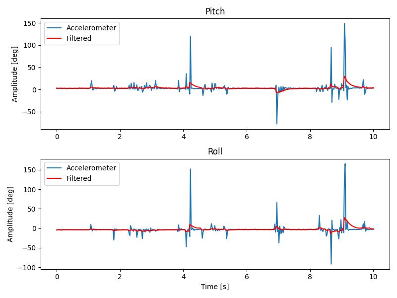

The low-pass filter cuts down on much of the high-frequency noise in the data. Interestingly, the ICM 20948 datasheet states that an integrated low-pass filter is already applied to the accelerometer, which explains why the noise was fairly tame even before my filtering.

Task 3: Gyroscope

To calculate pitch, roll, and yaw from the gyroscope's degrees per second, I implemented the following equations on the Artemis to integrate over time.

$${\theta }_g={\theta }_g+g_y\ast dt$$ $${\varphi }_g={\varphi }_g+g_x\ast dt$$ $${\psi }_g={\psi }_g+g_z\ast dt$$

dt = (micros() - last_time) / 1.e6; // us -> s
gy_pitch[n] = gy_pitch[n-1] - IMU.gyrY() * dt;
gy_roll[n] = gy_roll[n-1] + IMU.gyrX() * dt;
gy_yaw[n] = gy_yaw[n-1] + IMU.gyrZ() * dt;

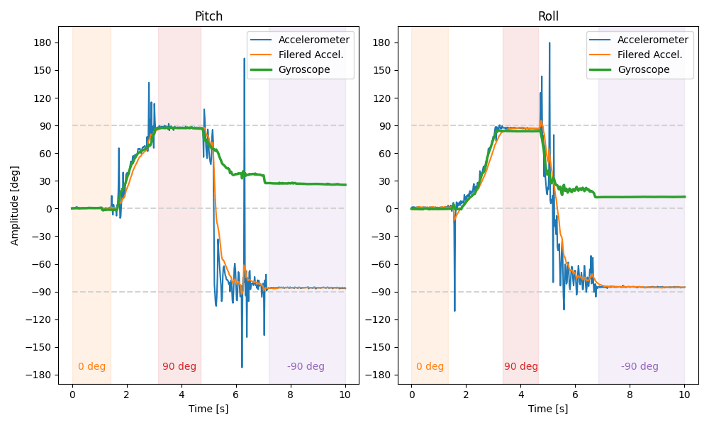
As with the accelerometer earlier, I tested the calculations by inducing pitches and rolls of 0, -90, and 90 degrees. Plotting the gyroscope measurements, I observed that:

1. the gyroscope data is significantly less noisy, even when compared to the filtered accelerometer data
2. the gyroscope drifts over time

To create a single, reliable signal, I combined the gyroscope and filtered accelerometer using a complimentary filter, defined by the equations:

$$\theta =(\theta +{\dot{\theta }}_{g}dt)(1-\gamma )+{\theta }_a\gamma$$ $$\varphi =(\varphi +{\dot{\varphi }}_{g}dt)(1-\gamma )+{\varphi }_a\gamma$$

Here, $\gamma$ is a weighting coefficient between the accelerometer and the gyroscope. Because the accelerometer is more accurate, I chose to use the gyroscope only sparingly by setting $\gamma$ to 0.9.

compliment_pitch[n] = (1 - GAMMA) * gy_pitch[n] + GAMMA * filtered_pitch[n];
compliment_roll[n] = (1 - GAMMA) * gy_roll[n] + GAMMA * filtered_roll[n];

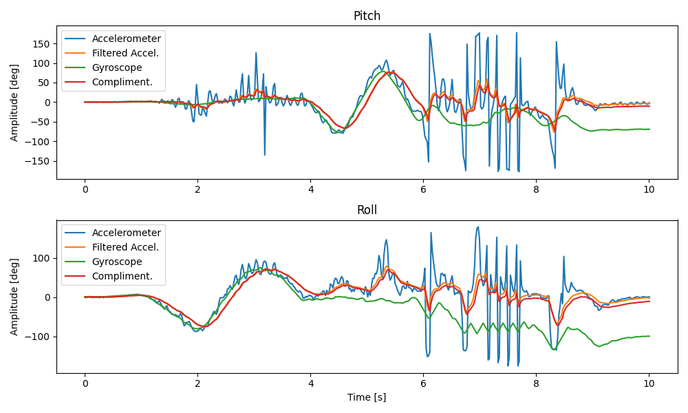
Moving the IMU in various ways (some slow, some rapid) revealed that the complimentary filter tends to stay accurate over time, avoiding the drift of the gyroscope, but is also not too quick to react to sudden vibrations. This makes the complimentary signal very reliable.

Task 4: Sample Data

Without any delay in main Artemis control loop, I achieved an IMU sampling rate of roughly 250 Hz. Without the sensor, the Artemis would be able to run at 48 Mhz. To prevent the IMU from blocking the Artemis, I changed the main loop to store IMU data only when it's ready and a global RECORD_IMU flag is set.

// In loop():
while (central.connected()) {
    // Record data only when a flag is set
    if (RECORD_IMU && IMU.dataReady()) {
        record_data();
    }

The function record_data() performs all the previously described calculations needed to find pitch, roll, and yaw from the IMU data. The RECORD_IMU flag is managed by new Artemis commands, replacing the data collection commands I used in this and previous labs.

// In handle_command():
case START_IMU_DATA:
    Serial.println("Recording IMU data...");
    digitalWrite(LED_BUILTIN, HIGH);
    RECORD_IMU = true;
    break;

case STOP_IMU_DATA:
    RECORD_IMU = false;
    digitalWrite(LED_BUILTIN, LOW);
    Serial.println("Stopped recording IMU data");
    break;

I could then call SEND_IMU_DATA in Python.

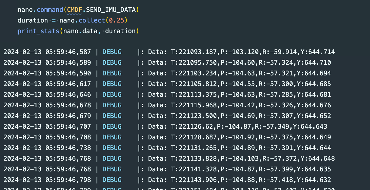
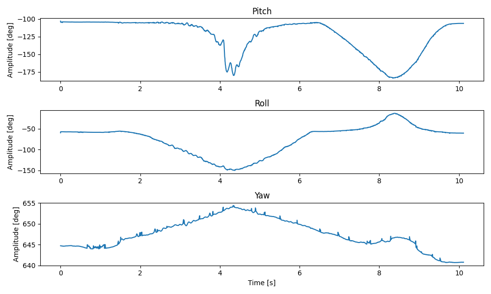
To store data, I used three float arrays, one for each of pitch, roll, and yaw. It makes most sense to store these three values separately and as floats so I can perform other calculations with them in the future. This is preferable to compacting the data into strings or the like.

Three float arrays each take up one third of the 384 KiB of Artemis memory. That equates to roughly 33,000 points of combined data. At the IMU's effective sampling rate of 250 Hz, filling that memory would take 132 seconds or just over 2 minutes. That's pretty good! In practice, though, these arrays aren't the only data in memory, so the real total sampling time will be somewhat lower and dependent on a variety of other factors.

Task 5: Record a Stunt

The last task was to check out our RC car. After driving it around a bit, the car felt quick. It can turn on the spot and flip due to its own torque when changing directions. Fitted with an Artemis, the little car will surely make a great robot.

Conclusion

This lab gave me an opportunity to work with a real sensor and experience real constraints. I'm excited to put my IMU recording system to the test on the RC car when we attach the Artemis.